library(fisheriescape)
library(gslSpatial)
library(terra)
library(ggplot2)
library(tidyterra)
library(dplyr)
Load example files and a 10 x 10 km2 hexagonal grid
- crab An example data set of snow crab fishing data
- fa.poly A shapefile of snow crab fishing area polygons
- grid A 10 x 10 km2 hexagonal grid sourced from https://gcgeo.gc.ca/geonetwork/metadata/eng/572f6221-4d12-415e-9d5e-984b15d34da4
df<-crab
fa.poly<-terra::vect(system.file("extdata/sample.fa.poly.shp", package="fisheriescape"))

grid<-gslSpatial::get_shapefile('hex')
grid<-terra::crop(grid,ext(fa.poly)*1.05)
Site score
First, select distinct rows by variable ‘event.id’.
df.ss<-distinct_at(df,vars('event.id'),.keep_all = T)
df.ss<-df.ss[-which(is.na(df.ss$x)|is.na(df.ss$y)),]

ggplot()+
  geom_spatvector(data=fa.poly,fill='white')+
  geom_spatvector(data=grid,fill=NA)+
  geom_point(data=df.ss,aes(x,y))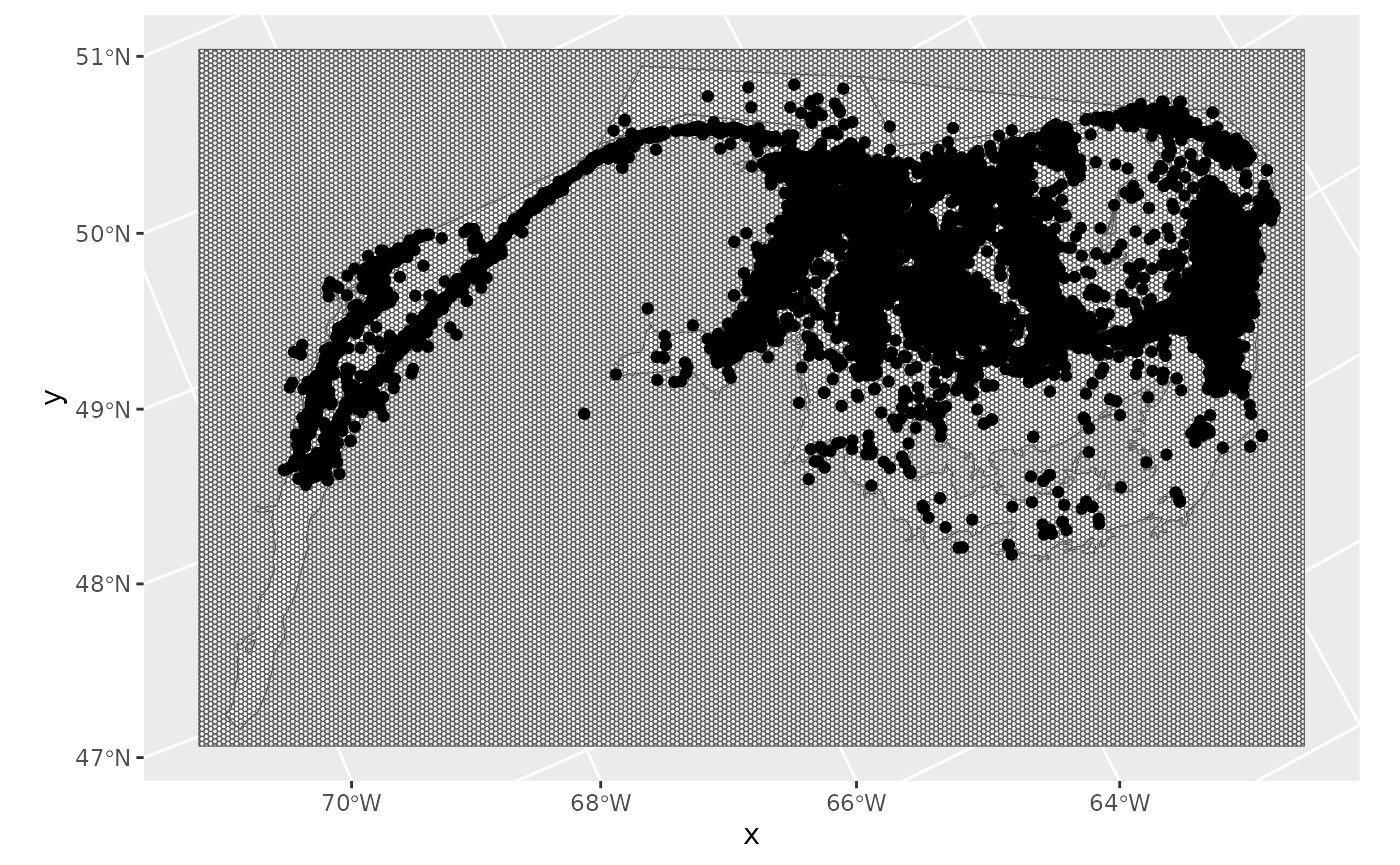
Next, use function fs_site_score. This function first
counts the number of fishing events per grid cell (hexagon) by standard
week and year. Then it calculates the mean number of fishing events by
standard week for each grid cell. Finally, it calculates the
site score of each grid cell by dividing the mean
number of fishing events in each grid cell by the mean number of fishing
events in each grid cell summed by fleet and standard week.
ss<-suppressMessages(fs_site_score(df.ss,fa.poly,grid=grid))# be patient
head(ss)
summary(ss)
#> # A tibble: 6 × 7
#> # Groups: fleet, sw [5]
#> GRID_ID sw tot.count.hex av.count.hex fleet sum.av.count.fleet site.score
#> <chr> <chr> <int> <dbl> <chr> <dbl> <dbl>
#> 1 ATW-1161 19 1 0.2 NA NA NA
#> 2 ATW-1161 20 2 0.4 NA NA NA
#> 3 ATW-1161 21 2 0.4 NA NA NA
#> 4 ATX-1161 21 1 0.2 NA NA NA
#> 5 ATY-1137 15 1 0.2 NA NA NA
#> 6 ATY-1143 13 1 0.2 NA NA NA
#> GRID_ID sw tot.count.hex av.count.hex
#> Length:16202 Length:16202 Min. : 1.000 Min. : 0.200
#> Class :character Class :character 1st Qu.: 1.000 1st Qu.: 0.200
#> Mode :character Mode :character Median : 2.000 Median : 0.400
#> Mean : 2.425 Mean : 0.485
#> 3rd Qu.: 3.000 3rd Qu.: 0.600
#> Max. :58.000 Max. :11.600
#>
#> fleet sum.av.count.fleet site.score
#> Length:16202 Min. : 0.2 Min. :0.000301
#> Class :character 1st Qu.:141.0 1st Qu.:0.000602
#> Mode :character Median :454.0 Median :0.001171
#> Mean :374.7 Mean :0.005595
#> 3rd Qu.:512.6 3rd Qu.:0.002736
#> Max. :664.6 Max. :1.000000
#> NA's :117 NA's :117In the figure below, red grid cells had data points, but these points fall outside of the fishing area polygons, and so are not included in the site score calculations.
index<-which(grid$GRID_ID%in%unlist(ss[which(is.na(ss$sum.av.count.fleet)),'GRID_ID']))

ggplot()+
  geom_spatvector(data=fa.poly,fill='white')+
  geom_spatvector(data=grid,fill=NA)+
  geom_spatvector(data=grid[index,],fill='red')

ss<-ss[-which(is.na(ss$site.score)),]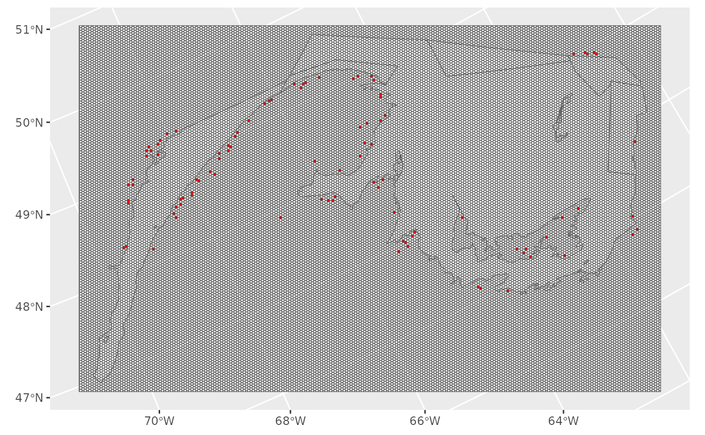
Pivot tables (pre-CEU steps)
Select distinct rows
df2<-distinct_at(df,vars('event.id','fleet','cfv','dateland','ctchdate',
                           'gear.amount',
                           'hours.fished'),.keep_all = T)

df2<-droplevels(df2)
names(df2)
#>  [1] "event.id"     "trip.id"      "cfv"          "dateland"     "ctchdate"
#>  [6] "latitude"     "longitude"    "year"         "sw"           "x"
#> [11] "y"            "fleet"        "gear.amount"  "hours.fished"
nrow(df2)
#> [1] 41154
Pivot 1
Function fs_pivot1 summarizes data by variables trip.id
and fleet. The resulting table contains the summed gear, maximum hours
(if applicable), and mean days (if applicable).
pivot1<-fs_pivot1(df2,
      keep.cols = c('cfv','year','sw'),
       gear.col='gear.amount',
       hour.col='hours.fished')
head(pivot1)
#>                           trip.id     fleet       cfv year sw sum.gear
#> 1    k6!ffg;2016-05-07;2016-05-07 GQ_CFA_12    k6!ffg 2016 18       NA
#> 2    k6!ffg;2016-05-15;2016-05-15 GQ_CFA_12    k6!ffg 2016 19       NA
#> 3    k6!ffg;2016-05-23;2016-05-23 GQ_CFA_12    k6!ffg 2016 21       NA
#> 4    k6!ffg;2016-05-28;2016-05-28 GQ_CFA_12    k6!ffg 2016 21       NA
#> 5 k6!8JJgk6;2016-05-14;2016-05-14 GQ_CFA_12 k6!8JJgk6 2016 19       NA
#> 6 k6!8JJgk6;2016-05-27;2016-05-27 GQ_CFA_12 k6!8JJgk6 2016 21       NA
#>   max.hours
#> 1        24
#> 2        24
#> 3        24
#> 4        24
#> 5        24
#> 6        24
summary(pivot1)
#>    trip.id             fleet                 cfv.V1            year
#>  Length:32302       Length:32302       Length:32302       Min.   :2013
#>  Class :character   Class :character   Class :character   1st Qu.:2014
#>  Mode  :character   Mode  :character   Mode  :character   Median :2015
#>                                                           Mean   :2015
#>                                                           3rd Qu.:2017
#>                                                           Max.   :2017
#>
#>       sw               sum.gear       max.hours
#>  Length:32302       Min.   :  1.0   Min.   :24
#>  Class :character   1st Qu.: 35.0   1st Qu.:24
#>  Mode  :character   Median : 71.0   Median :24
#>                     Mean   : 73.1   Mean   :24
#>                     3rd Qu.:100.0   3rd Qu.:24
#>                     Max.   :438.0   Max.   :24
#>                     NA's   :349
Now fill in the missing gear.amount with group averages.The user needs to choose the order of variables to group by that will be most appropriate for the fishery of interest. By the end of this step, there should be no missing gear.amount.
if(length(which(is.na(pivot1$sum.gear)))>0){
  pivot1<-fisheriescape::fs_fill_col(pivot1,group.cols=c('cfv','year','sw'),update.col = 'sum.gear',fun=mean)}

if(length(which(is.na(pivot1$sum.gear)))>0){
  pivot1<-fisheriescape::fs_fill_col(pivot1,group.cols=c('cfv','year'),update.col = 'sum.gear',fun=mean)}

if(length(which(is.na(pivot1$sum.gear)))>0){
  pivot1<-fisheriescape::fs_fill_col(pivot1,group.cols=c('cfv'),update.col = 'sum.gear',fun=mean)}

if(length(which(is.na(pivot1$sum.gear)))>0){
  pivot1<-fisheriescape::fs_fill_col(pivot1,group.cols=c('year','sw'),update.col = 'sum.gear',fun=mean)}

if(length(which(is.na(pivot1$sum.gear)))>0){
  pivot1<-fisheriescape::fs_fill_col(pivot1,group.cols=c('year'),update.col = 'sum.gear',fun=mean)}

if(length(which(is.na(pivot1$sum.gear)))>0){
  print('There are still NAs after filling gear according to current steps.')}
There are no longer NAs in gear.amount. If object pivot1 contained NAs in hours.fished, we would repeat the above step for hours.fished. However, we can see that there are no NAs in hours.fished.
summary(pivot1)
#>    trip.id             fleet                 cfv.V1            year
#>  Length:32302       Length:32302       Length:32302       Min.   :2013
#>  Class :character   Class :character   Class :character   1st Qu.:2014
#>  Mode  :character   Mode  :character   Mode  :character   Median :2015
#>                                                           Mean   :2015
#>                                                           3rd Qu.:2017
#>                                                           Max.   :2017
#>       sw               sum.gear        max.hours
#>  Length:32302       Min.   :  1.00   Min.   :24
#>  Class :character   1st Qu.: 35.00   1st Qu.:24
#>  Mode  :character   Median : 71.00   Median :24
#>                     Mean   : 73.03   Mean   :24
#>                     3rd Qu.:100.00   3rd Qu.:24
#>                     Max.   :438.00   Max.   :24
Pivot 2
Function fs_pivot2 summarizes data by user-specified
groups, which must include year, standard week (sw), fleet, and either
cfv or licence.
When trap.fishery==‘yes’, the resulting table contains the maximum gear, maximum hours (if applicable), and mean days (if applicable).
When trap.fishery!=‘yes’, the resulting table contains the mean gear, mean hours (if applicable), and mean days (if applicable).
pivot2<-fs_pivot2(pivot1,
                  trap.fishery='yes',
                  group.cols=c('cfv','fleet','year','sw'))
head(as.data.frame(pivot2))
#>      cfv     fleet year sw gear hours
#> 1 !2$82$ GQ_CFA_19 2013 29    8    24
#> 2 !2$82$ GQ_CFA_19 2013 30    8    24
#> 3 !2$82$ GQ_CFA_19 2014 29    8    24
#> 4 !2$82$ GQ_CFA_19 2014 30    8    24
#> 5 !2$82$ GQ_CFA_19 2014 31    8    24
#> 6 !2$82$ GQ_CFA_19 2015 29    8    24
summary(pivot2)
#>        cfv.V1          fleet                year           sw
#>  Length:14408       Length:14408       Min.   :2013   Length:14408
#>  Class :character   Class :character   1st Qu.:2014   Class :character
#>  Mode  :character   Mode  :character   Median :2015   Mode  :character
#>                                        Mean   :2015
#>                                        3rd Qu.:2017
#>                                        Max.   :2017
#>       gear            hours
#>  Min.   :  1.00   Min.   :24
#>  1st Qu.: 50.00   1st Qu.:24
#>  Median : 75.00   Median :24
#>  Mean   : 86.12   Mean   :24
#>  3rd Qu.:123.25   3rd Qu.:24
#>  Max.   :438.00   Max.   :24
Pivot 3
Function fs_pivot3 summarizes data by user-specified
groups, which must include year, standard week (sw), and fleet.
Grouping should not include either cfv or licence. A
parameter, “id.col”, needs to be specified as either cfv or licence.
When trap.fishery==‘yes’, the resulting table contains the number of distinct cfvs or licences (“n.vessels”), summed gear (“total.gear”), maximum hours (“soak.time”, if applicable), and mean days (“days”, if applicable).
When trap.fishery!=‘yes’, the resulting table contains the number of distinct cfvs or licences (“n.vessels”), summed gear (“total.gear”), mean hours (“soak.time”, if applicable), and mean days (“days”, if applicable).
pivot3<-fs_pivot3(pivot2,
                  group.cols=c('fleet','year','sw'),
                  id.col='cfv',
                  trap.fishery='yes')
head(as.data.frame(pivot3))
#>       fleet year sw n.vessels total.gear soak.time
#> 1 GQ_CFA_12 2013 17         5        289        24
#> 2 GQ_CFA_12 2013 18       251      24551        24
#> 3 GQ_CFA_12 2013 19       240      22352        24
#> 4 GQ_CFA_12 2013 20       243      22422        24
#> 5 GQ_CFA_12 2013 21       244      24111        24
#> 6 GQ_CFA_12 2013 22       238      23771        24
summary(pivot3)
#>     fleet                year           sw              n.vessels
#>  Length:288         Min.   :2013   Length:288         Min.   :  1.00
#>  Class :character   1st Qu.:2014   Class :character   1st Qu.:  5.00
#>  Mode  :character   Median :2015   Mode  :character   Median : 15.00
#>                     Mean   :2015                      Mean   : 50.03
#>                     3rd Qu.:2016                      3rd Qu.: 35.00
#>                     Max.   :2017                      Max.   :312.00
#>    total.gear      soak.time
#>  Min.   :    1   Min.   :24
#>  1st Qu.:  266   1st Qu.:24
#>  Median :  989   Median :24
#>  Mean   : 4308   Mean   :24
#>  3rd Qu.: 2690   3rd Qu.:24
#>  Max.   :31734   Max.   :24
Seasons and Pivot 4
The function fs_pivot4 is a little different from the
previous “pivot” functions, as it performs a number of steps. It does
not yet have a lot of flexibility, and needs to be used with caution.
Don’t use this function for fisheries that need information to be
summarized by province in addition to by fleet.
Function fs_pivot4 first identifies the start and end of
the fishing season for each year and fleet, and calculates the
proportion of each week that fishing occurs. It then joins the
proportion of week fished to the output from function
fs_pivot3.
pivot4<-fs_pivot4(df=df2,
                  trap.fishery='yes',
          pivot3, #output from fs_pivot3
          fleet.col='fleet', #should match between df and pivot3
          prov.col=NULL,
          area.note.col=NULL)
head(as.data.frame(pivot4))
#>       fleet year sw n.vessels total.gear soak.time prop.week.fished
#> 1 GQ_CFA_12 2013 17         5        289        24        0.2857143
#> 2 GQ_CFA_12 2013 18       251      24551        24        1.0000000
#> 3 GQ_CFA_12 2013 19       240      22352        24        1.0000000
#> 4 GQ_CFA_12 2013 20       243      22422        24        1.0000000
#> 5 GQ_CFA_12 2013 21       244      24111        24        1.0000000
#> 6 GQ_CFA_12 2013 22       238      23771        24        1.0000000
summary(pivot4)
#>     fleet                year           sw              n.vessels
#>  Length:288         Min.   :2013   Length:288         Min.   :  1.00
#>  Class :character   1st Qu.:2014   Class :character   1st Qu.:  5.00
#>  Mode  :character   Median :2015   Mode  :character   Median : 15.00
#>                     Mean   :2015                      Mean   : 50.03
#>                     3rd Qu.:2016                      3rd Qu.: 35.00
#>                     Max.   :2017                      Max.   :312.00
#>    total.gear      soak.time  prop.week.fished
#>  Min.   :    1   Min.   :24   Min.   :0.1429
#>  1st Qu.:  266   1st Qu.:24   1st Qu.:1.0000
#>  Median :  989   Median :24   Median :1.0000
#>  Mean   : 4308   Mean   :24   Mean   :0.9201
#>  3rd Qu.: 2690   3rd Qu.:24   3rd Qu.:1.0000
#>  Max.   :31734   Max.   :24   Max.   :1.0000
Common effort unit (CEU)
For most fisheries, use function fs_calc_ceu with the
output from fs_pivot4 and follow the prompts. This function
cannot yet be applied to American lobster, NAFO 4T.
For snow crab, fs_calc_ceu uses the following steps to
calculate CEU:
- rope.soak.time = soak.time/24
- magnitude = total.gear
- intensity = magnitude X rope.soak.time
- pre.ceu = intensity X proportion.week.fished
- ceu = sum pre.ceu by fleet and standard week, then divide by the number of years examined
df.ceu<-fs_calc_ceu(pivot4)

head(df.ceu)
#> # A tibble: 6 × 3
#> # Groups: fleet [1]
#> fleet sw ceu
#> <chr> <chr> <dbl>
#> 1 GQ_CFA_12 14 5.6
#> 2 GQ_CFA_12 15 14.4
#> 3 GQ_CFA_12 16 3115.
#> 4 GQ_CFA_12 17 9688.
#> 5 GQ_CFA_12 18 15934.
#> 6 GQ_CFA_12 19 19271.Fisheriescape
The fisheriescape is the product of the site score multiplied by the CEU.
Join site score with CEU and calculate fisheriescape
df<-left_join(ss,df.ceu)
df$fs<-df$site.score*df$ceu
head(df)
#> # A tibble: 6 × 9
#> # Groups: fleet, sw [4]
#> GRID_ID sw tot.count.hex av.count.hex fleet sum.av.count.fleet site.score
#> <chr> <chr> <int> <dbl> <chr> <dbl> <dbl>
#> 1 ATY-1159 19 1 0.2 GQ_CF… 100 0.002
#> 2 ATY-1159 20 2 0.4 GQ_CF… 88.4 0.00452
#> 3 ATY-1159 21 2 0.4 GQ_CF… 70.4 0.00568
#> 4 ATY-1160 18 1 0.2 GQ_CF… 108. 0.00185
#> 5 ATY-1160 20 2 0.4 GQ_CF… 88.4 0.00452
#> 6 ATY-1160 21 2 0.4 GQ_CF… 70.4 0.00568
#> # ℹ 2 more variables: ceu <dbl>, fs <dbl>
summary(df) # a small number of missing fs or av.ceu is expected
#> GRID_ID sw tot.count.hex av.count.hex
#> Length:16085 Length:16085 Min. : 1.000 Min. : 0.2000
#> Class :character Class :character 1st Qu.: 1.000 1st Qu.: 0.2000
#> Mode :character Mode :character Median : 2.000 Median : 0.4000
#> Mean : 2.435 Mean : 0.4869
#> 3rd Qu.: 3.000 3rd Qu.: 0.6000
#> Max. :58.000 Max. :11.6000
#>
#> fleet sum.av.count.fleet site.score ceu
#> Length:16085 Min. : 0.2 Min. :0.0003009 Min. :1.143e-01
#> Class :character 1st Qu.:141.0 1st Qu.:0.0006019 1st Qu.:2.938e+03
#> Mode :character Median :454.0 Median :0.0011705 Median :1.593e+04
#> Mean :374.7 Mean :0.0055953 Mean :1.405e+04
#> 3rd Qu.:512.6 3rd Qu.:0.0027364 3rd Qu.:2.204e+04
#> Max. :664.6 Max. :1.0000000 Max. :2.506e+04
#> NA's :26
#> fs
#> Min. : 0.1143
#> 1st Qu.: 7.5413
#> Median : 9.1276
#> Mean : 15.3383
#> 3rd Qu.: 18.2553
#> Max. :143.2850
#> NA's :26
#Checks
tapply(df$fs,df$fleet,summary)
#> $GQ_CFA_12
#> Min. 1st Qu. Median Mean 3rd Qu. Max.
#> 0.4143 8.1690 9.9722 16.9195 21.3870 143.2850
#>
#> $GQ_CFA_12A
#> Min. 1st Qu. Median Mean 3rd Qu. Max.
#> 1.971 4.865 5.948 10.290 13.778 60.982
#>
#> $GQ_CFA_12E
#> Min. 1st Qu. Median Mean 3rd Qu. Max. NA's
#> 5.80 15.60 17.30 17.71 19.67 34.80 1
#>
#> $GQ_CFA_12F
#> Min. 1st Qu. Median Mean 3rd Qu. Max.
#> 4.146 6.551 10.681 13.903 17.337 62.720
#>
#> $GQ_CFA_17
#> Min. 1st Qu. Median Mean 3rd Qu. Max.
#> 3.463 4.810 9.104 12.020 14.886 76.920
#>
#> $GQ_CFA_19
#> Min. 1st Qu. Median Mean 3rd Qu. Max. NA's
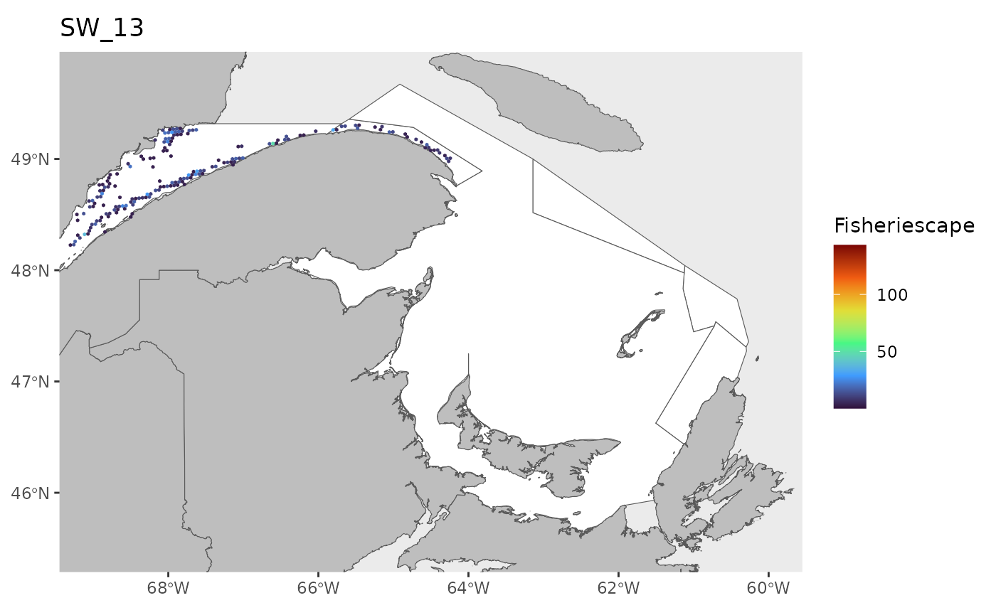
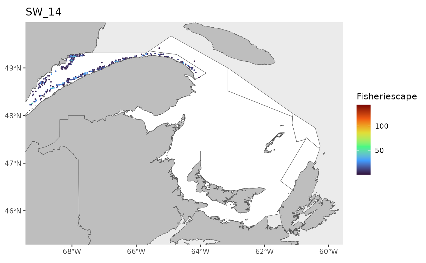
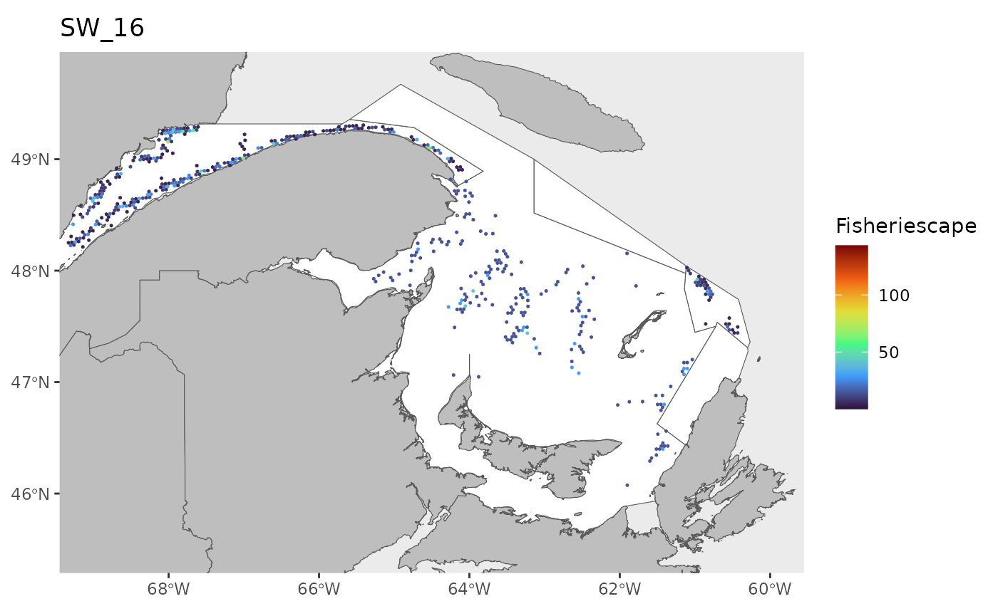
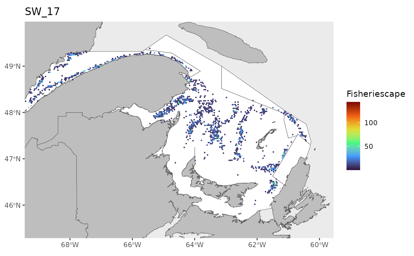
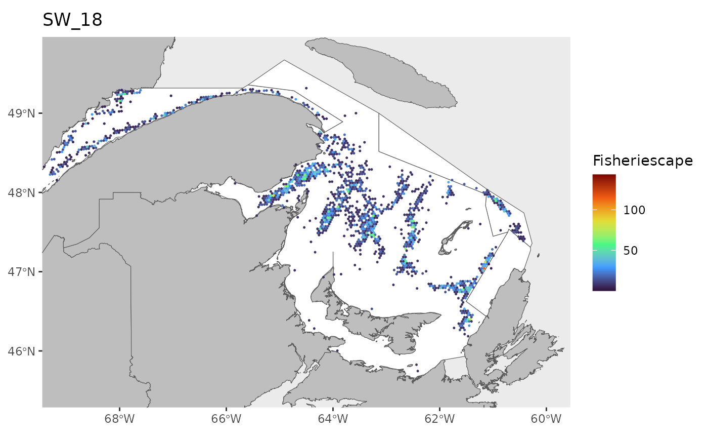
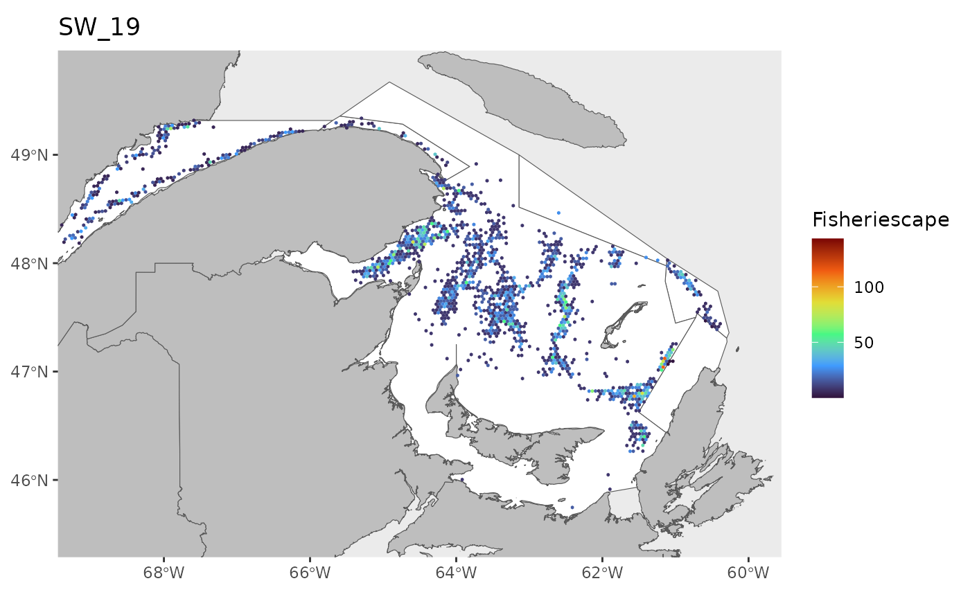
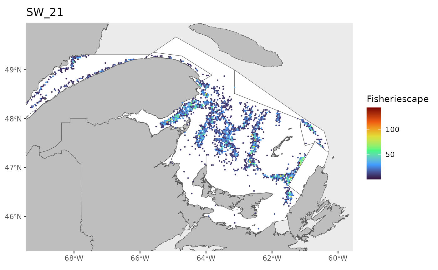
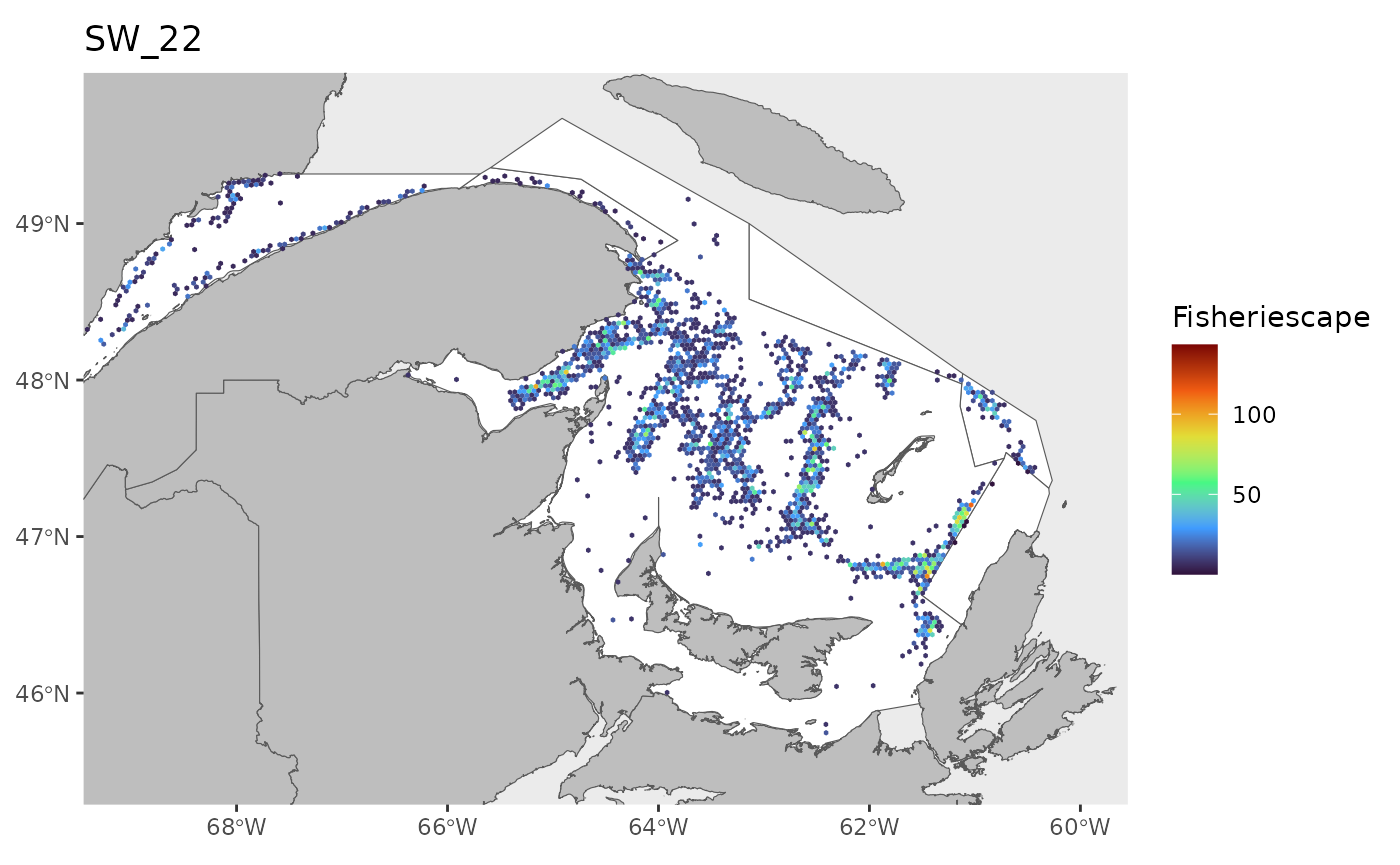
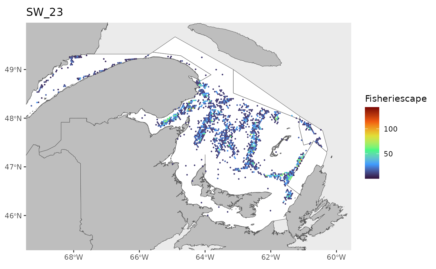
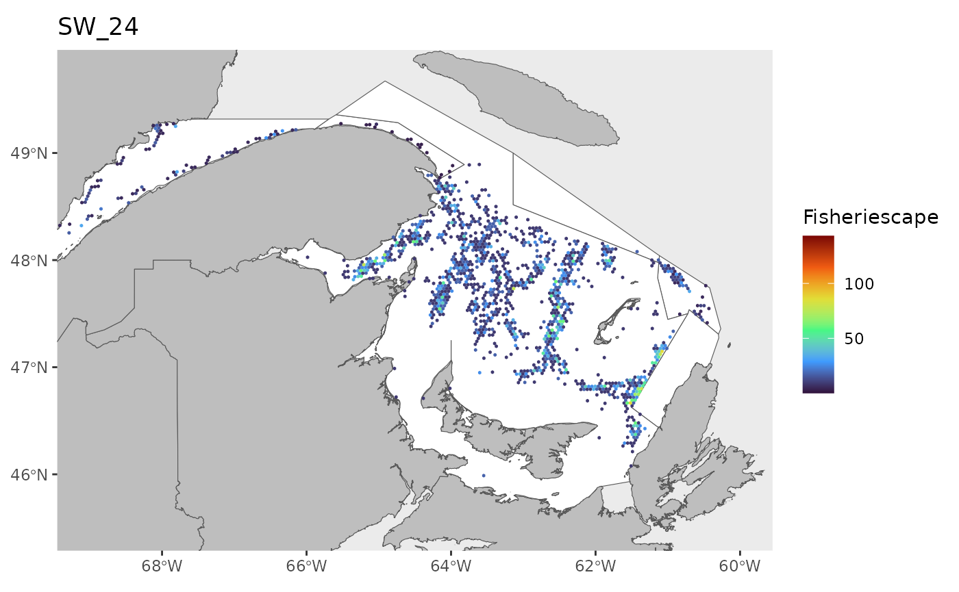
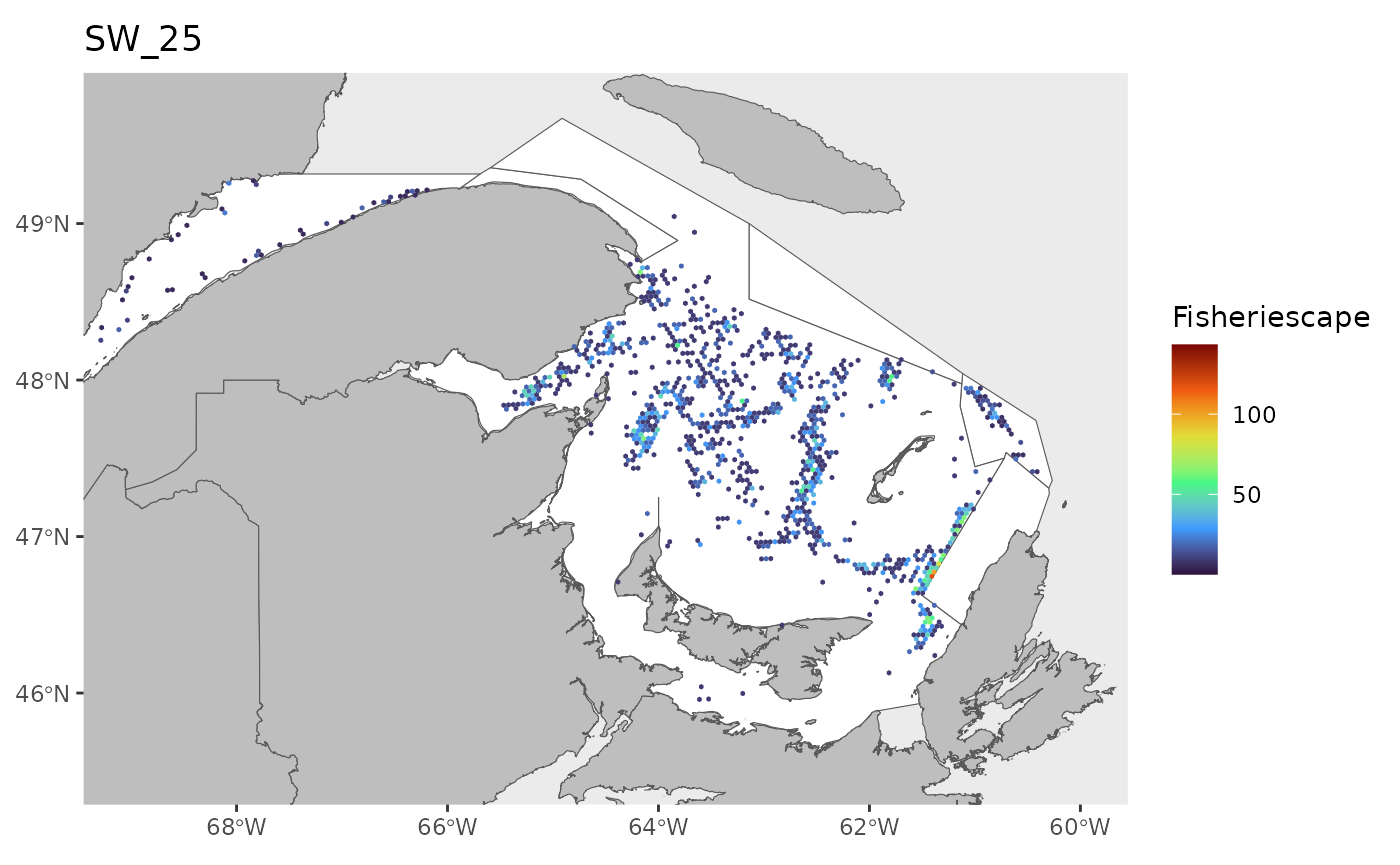
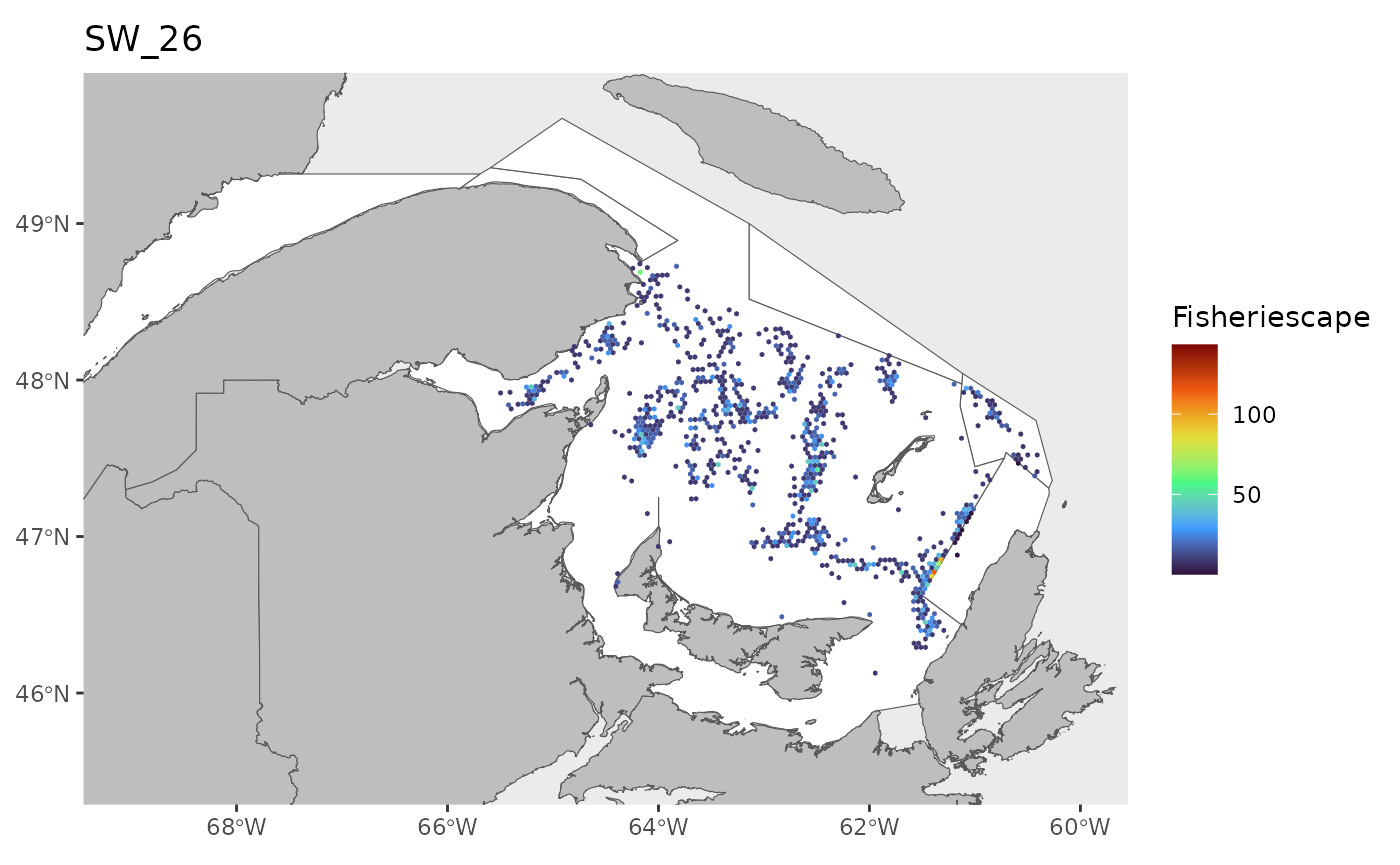
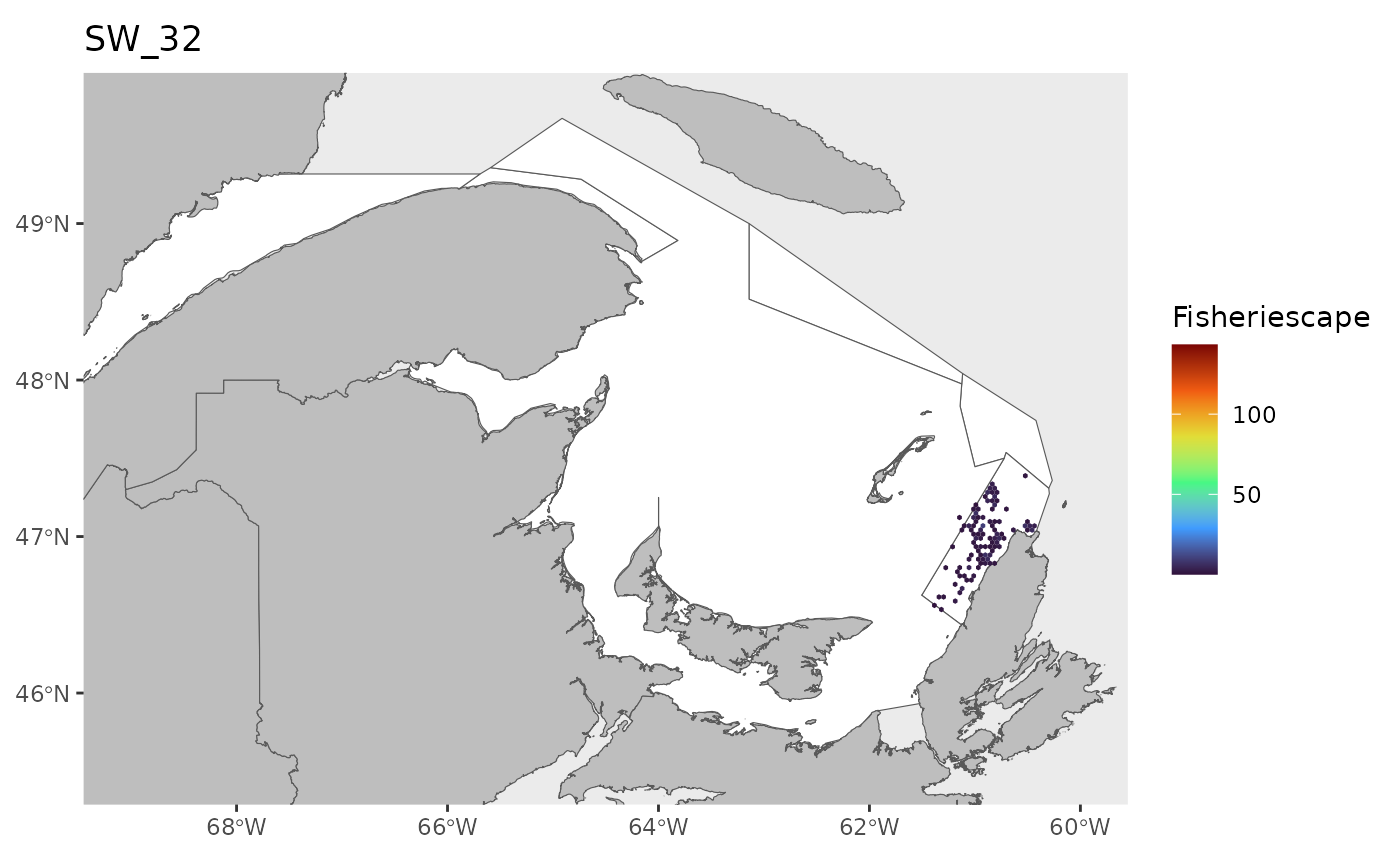
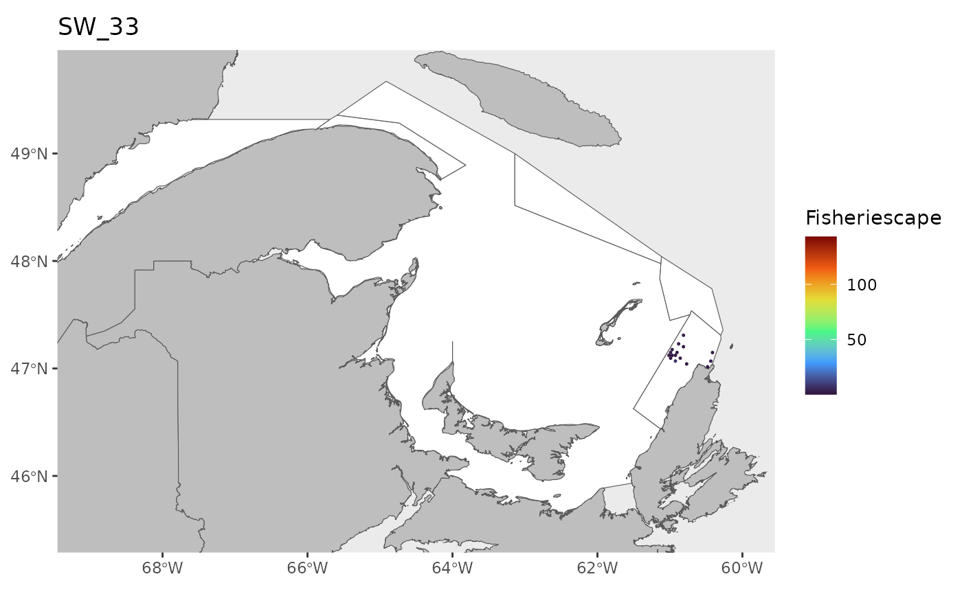
#> 0.1143 1.4726 2.9786 5.2980 6.7017 43.1890 25Plot
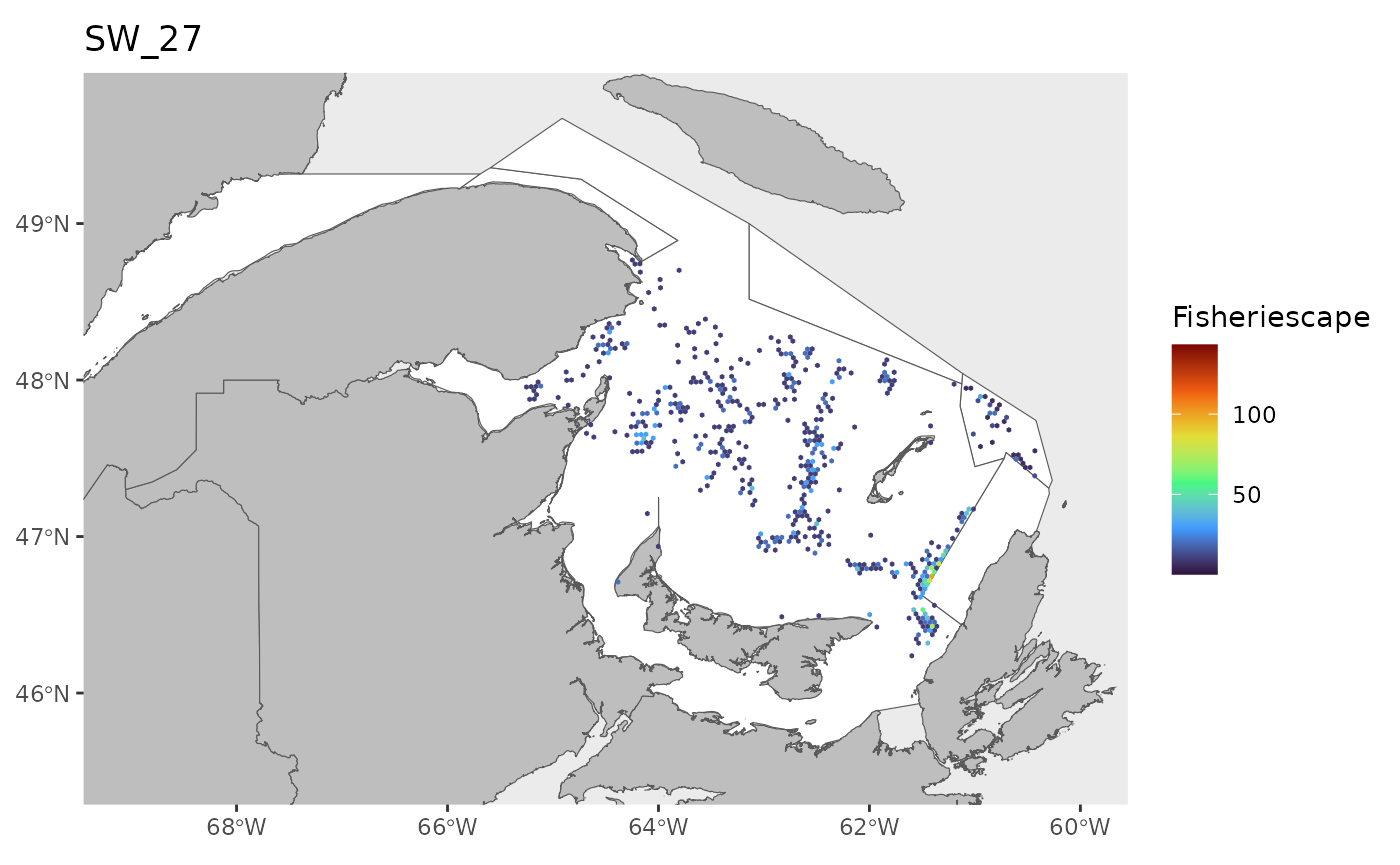
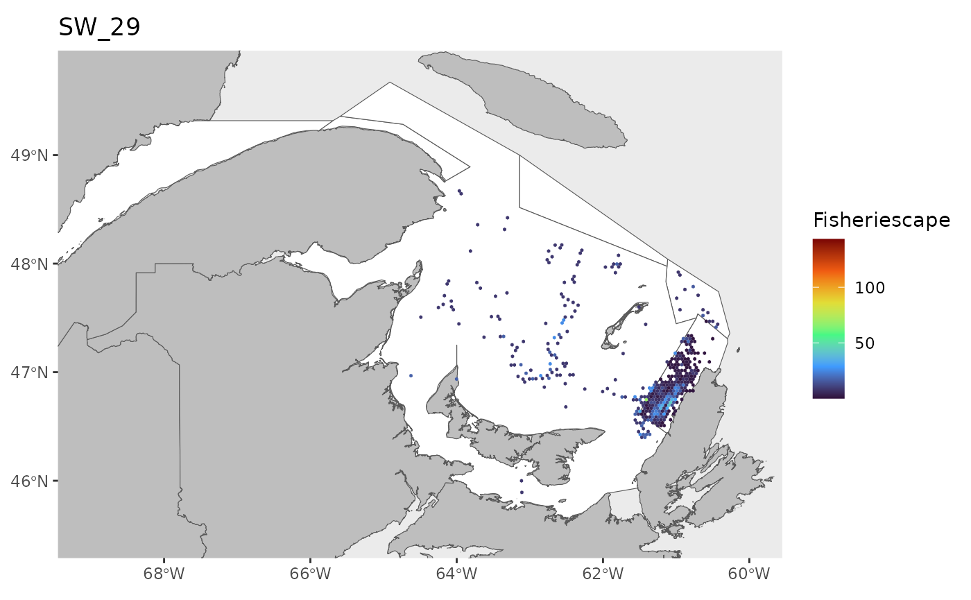
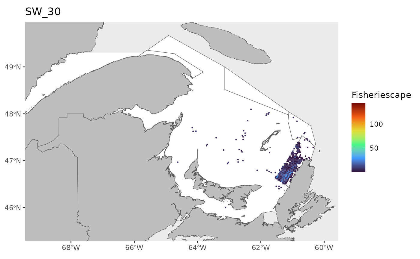
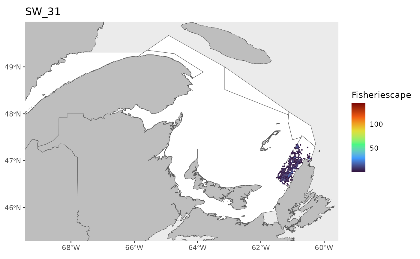
hex<-grid
naf<-get_shapefile('nafo.clipped')
naf<-project(naf,fa.poly)
names(naf)[1]<-'nafo'

coast<-gslSpatial::get_shapefile('coastline')
coast<-project(coast,fa.poly)

WEEKS<-sort(unique(df$sw))
fig.save='no'  # option to save file to specified path. If not 'yes', the figures will not be save and will only appear in the graphics window. If 'yes', the figures will be saved to the specified path, but will not be printed in the graphics window.
path.results<-'....' #path to store figures if fig.save=='yes'

for(i in 1:length(WEEKS)){
  dat<-df[which(df$sw==WEEKS[i]),]
  index<-which(is.na(dat$fs))
  if(length(index)>0){dat<-dat[-index,]}

  if(nrow(dat)>0){
    hex.out<-hex[which(hex$GRID_ID%in%unique(dat$GRID_ID)),]
    hex.out<-merge(hex.out,dat)

    pl<-ggplot()+
      geom_spatvector(data=fa.poly,fill='white')+
          geom_spatvector(data=coast,fill='grey')+
      geom_spatvector(data=hex.out,aes(fill=fs),col=NA)+
      scale_fill_viridis_c(direction=1,
                           option='turbo',
                           name="Fisheriescape",
                           limits = c(min(df$fs,na.rm=TRUE), max(df$fs,na.rm=TRUE)))+
      coord_sf(crs='epsg:4269',datum='epsg:4269',xlim=c(-69,-60),ylim=c(45.5,49.75))+
      ggtitle(paste0('SW_',WEEKS[i]))+
      theme(panel.grid.major = element_blank(),
            panel.grid.minor = element_blank())

   if(fig.save=='no'){print(pl)}else{ggsave(pl,
                          file = paste0(path.results,'FS_SW', WEEKS[i], '.jpg', sep = ''),
                          units = 'in', dpi = 600,height=4,width=6)}
  }
}